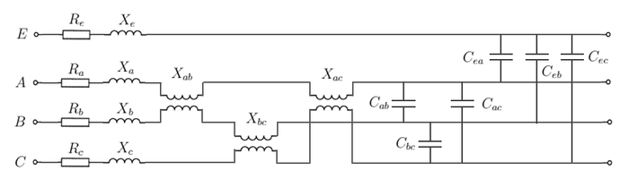
Figure 1. Circuit representation of a multi-conductor line segment
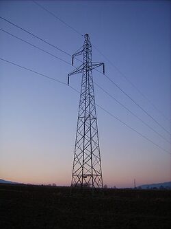
Figure 2. Three-phase, single-circuit tower line (image courtesy of
Wikipedia)
Consider the three-phase, single circuit tower line in Figure 2, which shows three phase conductors and an earth wire. A segmental length of this multi-conductor system can be represented by the equivalent circuit in Figure 1 above.
We can see that in a multi-conductor system, there is mutual coupling between the phase conductors (a, b and c), represented by the shunt inductances and capacitances. Note that there could also be resistive coupling between phases, but this is not shown in Figure 2 since resistive coupling is normally assumed to be negligible in overhead lines (i.e. shunt conductances G = 0).
This equivalent circuit can be represented as two  matrices (where n is the number of conductors in the system), one representing the series impedance
 ![{\displaystyle [Z]\,}](https://wikimedia.org/api/rest_v1/media/math/render/svg/5067b5d6d581b19e078d8c1d5a0b97bb0a373a5b) and the other representing the shunt admittance
and the other representing the shunt admittance ![{\displaystyle [Y]\,}](https://wikimedia.org/api/rest_v1/media/math/render/svg/01412c6c505c0e62440bd89cb84c00de04d6da8d) .
.
For example, the four conductor system in Figure 2 has the  series impedance matrix:
![{\displaystyle [Z]=\left[{\begin{matrix}Z_{aa}&Z_{ab}&Z_{ac}&|&Z_{ae}\\Z_{ba}&Z_{bb}&Z_{bc}&|&Z_{be}\\Z_{ca}&Z_{cb}&Z_{cc}&|&Z_{ce}\\--&--&--&|&--\\Z_{ea}&Z_{eb}&Z_{ec}&|&Z_{ee}\end{matrix}}\right]\,}](https://wikimedia.org/api/rest_v1/media/math/render/svg/8b99df43a0ccf27e31891fa8be0e91d64209dfbc)
And the shunt admittance matrix:
![{\displaystyle [Y]=\left[{\begin{matrix}Y_{aa}&Y_{ab}&Y_{ac}&|&Y_{ae}\\Y_{ba}&Y_{bb}&Y_{bc}&|&Y_{be}\\Y_{ca}&Y_{cb}&Y_{cc}&|&Y_{ce}\\--&--&--&|&--\\Y_{ea}&Y_{eb}&Y_{ec}&|&Y_{ee}\end{matrix}}\right]\,}](https://wikimedia.org/api/rest_v1/media/math/render/svg/cc5f732b4148fef09f52bc3039332455554e90eb)
Elements in the series impedance and shunt admittance matrices are complex quantities of the form:  and
and  .
.
For most types of analyses, we can assume that the elements in the series impedance and shunt admittance matrices are constant terms without introducing too much error. These matrices are commonly called the overhead line constants and are calculated based on the overhead line conductor properties and cross-sectional geometry.
Assumptions
The following assumptions are made to simplify the line constants calculations:
- There is uniform current distribution in the conductor, thus conductor stranding is not taken into account
- The earth is flat along the length of the transmission line, i.e. earth curvature not allowed for
- Uniform soil conditions along the length of the transmission line, i.e. constant soil resistivity
Series Impedance Matrix
The lengths and angles referred to in the calculations below are all based on the geometry of two aerial conductors i and k shown in Figure 3.
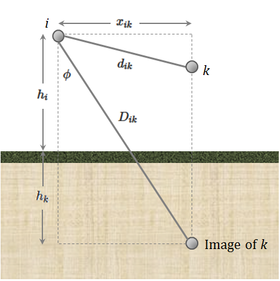
Figure 3. Geometry of two aerial conductors
Self Impedance Terms
The self impedance of an aerial conductor is calculated as follows:

where  is the internal resistance of the conductor (
 /km)
/km)
 is the internal reactance of the conductor (/km)
 is the geometrical reactance (/km)
 and
and  are the Carson earth correction factors (/km) - see separate section below
When skin effect is not taken into account, the internal resistance is simply the DC resistance of the conductor  .
.
The internal reactance of the conductor depends on the type of conductor used, e.g. solid conductor (AAAC) vs a tubular conductor, where there is a non-conducting reinforcing material in the centre of the conductor (ACSR).
The reactance of a solid conductor (in /km) is calculated as follows:

where  is the permeability of free space (
 H/m)
H/m)
The reactance of a tubular / hollow core conductor (in /km) is calculated as follows:
![{\displaystyle X_{int}^{'}=1000\times j\omega {\frac {\mu _{0}}{2\pi }}\left[{\frac {q^{4}}{(r^{2}-q^{2})^{2}}}\cdot \ln {\frac {r}{q}}\cdot {\frac {3q^{2}-r^{2}}{4(r^{2}-q^{2})}}\right]}](https://wikimedia.org/api/rest_v1/media/math/render/svg/dbee58fc7f3c9d53ff6da355411207e51287ff60)
where  is the nominal angular frequency of the system (rad/s)
 is the inner radius of the tubular conductor (m)
 is the outer radius of the tubular conductor (m)
The geometrical reactance (in /km) can be calculated as follows:

where  is the radius of the conductor (m)
 is the height of the conductor above ground level (m)
Mutual Impedance Terms
The mutual impedance between any two aerial conductors is calculated as follows:

where  is the geometrical reactance between conductors i and k (/km)
 and
and  are the Carson earth correction factors (/km) - see separate section below
The geometrical reactance between conductors i and k (in /km) can be calculated as follows:

where  is the distance between conductor i and conductor k (m)
 is the distance between conductor i and the image of conductor k in the ground (m)
Carson Earth Correction Factors
Because the earth/ground is a conducting medium, it has an effect on the magnetic field produced by the current flowing in an aerial conductor. During unbalanced operation or in single-phase earth return (SWER) systems, the earth also acts as a conductor for currents to return to the source.
The Carson earth correction factors are infinite series (with terms that repeat in groups of four):
![{\displaystyle \Delta R_{ii}^{'}=4\omega \times 10^{-4}\left({\frac {\pi }{8}}-b_{1}a\cos {\phi }+b_{2}\left[(c_{2}-\ln {a})a^{2}\cos {2\phi }+\phi a^{2}\sin {2\phi }\right]+b_{3}a^{3}\cos {3\phi }-d_{4}a^{4}\cos {4\phi }-b_{5}a^{5}cos{5\phi }+b_{6}\left[(c_{6}-\ln {a})a^{6}\cos {6\phi }+\phi a^{6}\sin {6\phi }\right]+b_{7}a^{7}\cos {7\phi }-d_{8}a^{8}\cos {8\phi }+\dots \right)}](https://wikimedia.org/api/rest_v1/media/math/render/svg/41621845396f908ffec1e00e06382ce6d9efdf87)
![{\displaystyle \Delta X_{ii}^{'}=4\omega \times 10^{-4}\left({\frac {1}{2}}(0.6159315-\ln {a})+b_{1}a\cos {\phi }-d_{2}a^{2}\cos {2\phi }+b_{3}a^{3}\cos {3\phi }-b_{4}\left[(c_{4}-\ln {a})a^{4}\cos {4\phi }+\phi a^{4}\sin {4\phi }\right]+b_{5}a^{5}\cos {5\phi }-d_{6}a^{6}\cos {6\phi }+b_{7}a^{7}cos{7\phi }-b_{8}\left[(c_{8}-\ln {a})a^{8}\cos {8\phi }+\phi a^{8}\sin {8\phi }\right]+\dots \right)}](https://wikimedia.org/api/rest_v1/media/math/render/svg/b1acda55cf9fe0371078cab99e01650f9414f2cc)
where 
 with
with  ,
,  and
and  alternating in groups of 4, i.e.
  for i=1,2,3,4,
  for i=5,6,7,8, for i=9,10,11,12 and so on
 with
with 

 is the soil resistivity (
 )
) for self impedance terms and
  for mutual impedance terms
Note that this formulation is only valid if  .
.
Shunt Admittance Matrix
The self potential terms of the shunt admittance matrix are calculated as follows:

where is the radius of the conductor (m)
- is the height of the conductor above ground level (m)
 is the permittivity of free space (
 F/m)
F/m)
The mutual potential terms of the shunt admittance matrix are calculated as follows:

where is the distance between conductor i and conductor k (m)
- is the distance between conductor i and the image of conductor k in the ground (m)
Kron Reduction
Assuming that the voltage in the earth conductors are zero (i.e. earth is the reference voltage), the earth conductors in the primitive series impedance and shunt admittance matrices can be eliminated by means of a Kron Reduction.
Code
Refer to this Github project for an open-source Python implementation of a line constants calculation routine.


