Introduction
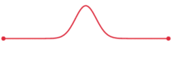
Figure 1. Travelling wave along a line (image courtesy of
Wikipedia)
A travelling wave on a transmission line is a transient disturbance that that moves along the line at a constant speed yet maintains its shape (see Figure 1). Examples include lightning surges, switching transients, faults, etc.
In this article, we will derive various time-domain models for travelling waves on transmission lines, starting from the simplest case of the lossless single-phase line, then building to a generic lossy single-phase line. The derivation of the model is also looked at starting from the frequency-domain, showing the symmetry of the frequency and time-domain models. Finally, the considerations required to extend the model to a multi-conductor line is discussed.
This article provides the theoretical background for the travelling wave model. Actual implementations of the model suitable for use in computer simulations (i.e. discrete-time) can be found in the following articles:
Lossless Single-Phase Lines
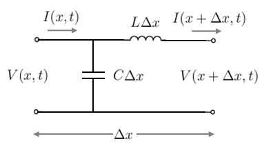
Figure 2. Travelling wave line model - Small Segment from a lossless single-phase line
Consider the small segment of length  metres from a lossless single-phase transmission line shown in Figure 2.
Notice that the model is similar to that of the classical distributed parameter line model, except that in this model, the voltages and currents are functions of both distance  and time
  and are real, not phasor quantities. In the classical distributed parameter line model, the voltages and currents are evaluated at steady-state and are only functions of distance .
Derivation of Voltage and Current Equations
Analysing this circuit using Kirchhoff's voltage law and Kirchhoff's current law, we can get the following pair of equations:


Notes:
- 1. The voltage across an inductor is
 and the current through a capacitor is
  .
.
- 2. Partial derivatives are used because the voltages and currents are functions of both time and distance.
Re-arranging the above equations, we get:


Taking the limit as  yields the well known Telegrapher's equations:
 ... Equ. (1)
 ... Equ. (2)
Differentiating the voltage equation with respect to x and the current equation with respect to t:
 ... Equ. (3)
 ... Equ. (4)
Now substituting Equ. (4) into Equ. (3), we get:
 ... Equ. (5)
Similarly, we could have differentiated the current equation with respect to x and the voltage equation with respect to t and then solved for the current equation:
 ... Equ. (6)
The pair of equations (5) and (6) above are referred to as the transmission line wave equations.
The general solution to either of these equations can be found using d'Alembert's formula:


where  is the velocity of propagation (m/s).
 and
and  are arbitrary current functions of time.
 and
and  are arbitrary voltage functions of time.
Using the current equation above, we can solve for the voltage equation as follows (see here for the full derivation):
![{\displaystyle v(x,t)=Z_{c}\left[i^{+}(x-vt)-i^{-}(x+vt)\right]\,}](https://wikimedia.org/api/rest_v1/media/math/render/svg/a511e20a7e574b6c3e7b3d2966f26f7ed951650a)
where  is the characteristic impedance (Ohms)
Significance of + and - Equations
So we have the pair of voltage and current equations:
![{\displaystyle V(x,t)=Z_{c}\left[i^{+}(x-vt)-i^{-}(x+vt)\right]\,}](https://wikimedia.org/api/rest_v1/media/math/render/svg/dbf43663b38d993aaa6ac5e01eb0f321d39d9413)
What is the significance of  and
and  ?
?
Consider that time t=0s, the function  represents an arbitrary waveform / shape distributed in space along the transmission line. For example, it could look like this:
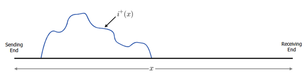
Figure 3. Arbitrary waveform

at time t = 0s
Now consider what happens at time t=1s, the function  has the same shape as the function above, but is translated to the right by
  metres:
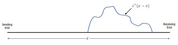
Figure 4. Arbitrary waveform

at time t = 1s
What we can conclude is that the function is an arbitrary waveform that maintains its shape but moves in the direction of the receiving end with increasing time at speed m/s. This is called a forward travelling wave.
We can use similar logic to conclude that the function is an arbitrary waveform that moves in the opposite direction (i.e. in the direction of the sending end). This is referred to as a backward travelling wave.
Generic Lossy Single-Phase Lines
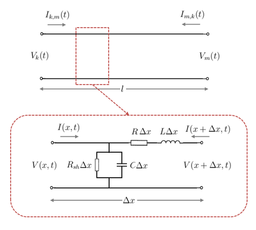
Figure 5. A generic single-phase distributed parameter line model
Consider the generic single-phase distributed parameter line model of length  metres shown in Figure 5. Analysing the circuit using Kirchhoff's laws as we did previously in the lossless case, we can get:


Where  is the shunt conductance.
Differentiating the voltage equation with respect to x and the current equation with respect to t:
 ... Equ. (7)
 ... Equ. (8)
Substituting Equ. (8) into Equ. (7), we get:
 ... Equ. (9)
If we were to set R = G = 0 in the equation above, then we would get the same transmission line wave equation as Equ. (5) in the lossless case.
However, while there is a general solution to the lossless line using d'Alembert's formula (as shown earlier), the generic lossy line does not have a neat, closed-form solution.
Frequency Domain Derivation
In the preceding sections, the travelling wave model was developed purely in the time-domain. Another way of looking at the travelling wave model is to derive it first in the frequency domain and then convert it to the time-domain. Recall from the steady-state (frequency domain) distributed parameter model that the sending end voltage and current can be related to the receiving end quantities as follows:
![{\displaystyle \left[{\begin{matrix}{\boldsymbol {V_{s}}}\\\\{\boldsymbol {I_{s}}}\end{matrix}}\right]=\left[{\begin{matrix}\cosh({\boldsymbol {\gamma }}l)&{\boldsymbol {Z}}_{c}\sinh({\boldsymbol {\gamma }}l)\\\\{\frac {1}{{\boldsymbol {Z}}_{c}}}sinh({\boldsymbol {\gamma }}l)&\cosh({\boldsymbol {\gamma }}l)\end{matrix}}\right]\left[{\begin{matrix}{\boldsymbol {V_{r}}}\\\\{\boldsymbol {I_{r}}}\end{matrix}}\right]\,}](https://wikimedia.org/api/rest_v1/media/math/render/svg/84c751fe40fbb9e608b1835a0512c90917157eaa)
where  is the propagation constant (
 )
)
 is the characteristic impedance (
 )
) and
and  are the series impedance and shunt admittance respectively
With some straightforward algebraic manipulation, the steady-state equations above can be represented in the following form:
 ... Equ. (10)
The time-domain model can be derived by calculating the inverse Fourier transform of Equ. (10).
In the lossless case (i.e. R = G = 0.), the propagation constant and characteristic impedance are as follows:


A property of Fourier transforms is that multiplying by a complex exponential in the frequency domain results in a time shift in the time domain. Therefore, taking the inverse Fourier transform of Equ. (10) for the lossless case, we get:

The lossless case above shows that the receiving end quantities are essentially time-shifted (past) versions of the sending end quantities, as was derived earlier using d'Alembert's formula.
In the general lossy case, the characteristic impedance is not a scalar constant (but rather a function of frequency  ) and the propagation constant does not lead to a simple time shift in the time-domain. Therefore, the inverse Fourier transform of Equ. (10) leads to a series of messy convolutions:
![{\displaystyle v_{r}(t)+z_{c}(t)*i_{r}(t)=\left[v_{s}(t)+z_{c}(t)*i_{s}(t)\right]*a(t)\,}](https://wikimedia.org/api/rest_v1/media/math/render/svg/6dc28c7b967b6e3bb92b47ab631c1ebf7e0291e6)
where  is the inverse Fourier transform of
 is the inverse Fourier transform of
As can be imagined, the convolution integrals in the equation above are not neatly solvable.
Multi-conductor Lines
The travelling wave line model for the single-phase lossless line can be extended to a multi-conductor line of n conductors by replacing the voltage and current quantities with  vectors, e.g. for a three-phase, three-conductor line:
![{\displaystyle {\boldsymbol {V}}(x,t)=\left[{\begin{matrix}{\boldsymbol {V_{a}}}(x,t)\\{\boldsymbol {V_{b}}}(x,t)\\{\boldsymbol {V_{c}}}(x,t)\end{matrix}}\right]\,}](https://wikimedia.org/api/rest_v1/media/math/render/svg/92a3e76d80ce7c7d76ac3ed4023ac1945258b092) ,
, ![{\displaystyle {\boldsymbol {I}}(x,t)=\left[{\begin{matrix}{\boldsymbol {I_{a}}}(x,t)\\{\boldsymbol {I_{b}}}(x,t)\\{\boldsymbol {I_{c}}}(x,t)\end{matrix}}\right]\,}](https://wikimedia.org/api/rest_v1/media/math/render/svg/0f0675967fbcd1e542f2af034e18bb212698b80e)
And the inductance and capacitance (per unit length) with  matrices to capture the mutual coupling between phases, e.g. for a three-phase, three-conductor line:
![{\displaystyle [L]=\left[{\begin{matrix}L_{aa}&L_{ab}&L_{ac}\\L_{ba}&L_{bb}&L_{bc}\\L_{ca}&L_{cb}&L_{cc}\end{matrix}}\right]\,}](https://wikimedia.org/api/rest_v1/media/math/render/svg/c96f736ed81e45dc57e37fd91eb6b4ad6481a00b)
![{\displaystyle [C]=\left[{\begin{matrix}C_{aa}&C_{ab}&C_{ac}\\C_{ba}&C_{bb}&C_{bc}\\C_{ca}&C_{cb}&C_{cc}\end{matrix}}\right]\,}](https://wikimedia.org/api/rest_v1/media/math/render/svg/40d5d9c126ab5c96a322b3b8238d941b040da843)
The transmission line wave equations for the single-phase model (see equations (5) and (6) above) can now be re-written for the multi-conductor model as follows:
![{\displaystyle {\frac {\partial ^{2}{\boldsymbol {V}}(x,t)}{\partial x^{2}}}=[L][C]{\frac {\partial ^{2}{\boldsymbol {V}}(x,t)}{\partial t^{2}}}\,}](https://wikimedia.org/api/rest_v1/media/math/render/svg/7d7010fead951cf098d8f148e870d3f2de0af174) ... Equ. (10)
... Equ. (10)
![{\displaystyle {\frac {\partial ^{2}{\boldsymbol {I}}(x,t)}{\partial x^{2}}}=[C][L]{\frac {\partial ^{2}{\boldsymbol {I}}(x,t)}{\partial t^{2}}}\,}](https://wikimedia.org/api/rest_v1/media/math/render/svg/b208c4aa9d0624f39268ab08b84be066a2ca2981) ... Equ. (11)
... Equ. (11)
Unlike the single-phase case, there is no general solution to the second-order differential equations (10) and (11) since the matrix product [L][C] is typically full (i.e. off-diagonals are non-zero). To solve these differential equations, a modal transformation is required to decouple the phases (refer to this section of the distributed parameter line article for more details on the modal transformation).
The voltage and current vectors are transformed from the phase domain to the modal domain by the transformation matrices ![{\displaystyle [T_{v}]\,}](https://wikimedia.org/api/rest_v1/media/math/render/svg/2838c4c191c867ff1627123f06beedcb05c2d2bd) and
and ![{\displaystyle [T_{i}]\,}](https://wikimedia.org/api/rest_v1/media/math/render/svg/e29111c511b58a6f5ac4f689dacee1e8f3027e50) , such that:
, such that:
![{\displaystyle {\boldsymbol {V}}(x,t)=[T_{v}]{\boldsymbol {V'}}(x,t)}](https://wikimedia.org/api/rest_v1/media/math/render/svg/43a11db8153ea987e2774742d77917a468c267a6)
![{\displaystyle {\boldsymbol {I}}(x,t)=[T_{i}]{\boldsymbol {I'}}(x,t)}](https://wikimedia.org/api/rest_v1/media/math/render/svg/33c02d41657c190a007b845bf19dbada2f5c8eac)
where  and
and  are the modal voltage and current vectors, i.e.
![{\displaystyle {\boldsymbol {V'}}(x,t)=\left[{\begin{matrix}{\boldsymbol {V_{0}}}(x)\\{\boldsymbol {V_{1}}}(x)\\{\boldsymbol {V_{2}}}(x)\end{matrix}}\right]\,}](https://wikimedia.org/api/rest_v1/media/math/render/svg/4af3d79bb6e1293ec559160f0a8375ac2bd66385) ,
, ![{\displaystyle {\boldsymbol {I'}}(x,t)=\left[{\begin{matrix}{\boldsymbol {I_{0}}}(x)\\{\boldsymbol {I_{1}}}(x)\\{\boldsymbol {I_{2}}}(x)\end{matrix}}\right]\,}](https://wikimedia.org/api/rest_v1/media/math/render/svg/7a38da1778238a8d5cf7eb5a6b9786fddc6708e0)
The transformation matrices and are selected such that they are the eigenvectors of [L][C] and [C][L] respectively (note that they have the same eigenvalues).
In the modal domain, equations (10) and (11) can be re-written as sets of decoupled equations, i.e.
![{\displaystyle \left[{\begin{matrix}{\frac {d^{2}{\boldsymbol {V_{0}}}(x,t)}{dx^{2}}}\\\\{\frac {d^{2}{\boldsymbol {V_{1}}}(x,t)}{dx^{2}}}\\\\{\frac {d^{2}{\boldsymbol {V_{2}}}(x,t)}{dx^{2}}}\end{matrix}}\right]=\left[{\begin{matrix}\lambda _{0}&&\\&\lambda _{1}&\\&&\lambda _{2}\end{matrix}}\right]\left[{\begin{matrix}{\frac {d^{2}{\boldsymbol {V_{0}}}(x,t)}{dt^{2}}}\\\\{\frac {d^{2}{\boldsymbol {V_{1}}}(x,t)}{dt^{2}}}\\\\{\frac {d^{2}{\boldsymbol {V_{2}}}(x,t)}{dt^{2}}}\end{matrix}}\right]\,}](https://wikimedia.org/api/rest_v1/media/math/render/svg/f81c3a0e8fcb1718ab6d665dac453314d71fbeb1) ... Equ. (12)
... Equ. (12)
![{\displaystyle \left[{\begin{matrix}{\frac {d^{2}{\boldsymbol {I_{0}}}(x,t)}{dx^{2}}}\\\\{\frac {d^{2}{\boldsymbol {I_{1}}}(x,t)}{dx^{2}}}\\\\{\frac {d^{2}{\boldsymbol {I_{2}}}(x,t)}{dx^{2}}}\end{matrix}}\right]=\left[{\begin{matrix}\lambda _{0}&&\\&\lambda _{1}&\\&&\lambda _{2}\end{matrix}}\right]\left[{\begin{matrix}{\frac {d^{2}{\boldsymbol {I_{0}}}(x,t)}{dt^{2}}}\\\\{\frac {d^{2}{\boldsymbol {I_{1}}}(x,t)}{dt^{2}}}\\\\{\frac {d^{2}{\boldsymbol {I_{2}}}(x,t)}{dt^{2}}}\end{matrix}}\right]\,}](https://wikimedia.org/api/rest_v1/media/math/render/svg/4ddc0f58c841bd75d1e7a5a9ad6da4be816cb1c2) ... Equ. (13)
... Equ. (13)
These modal differential equations can then be solved individually using d'Alembert's formula. For example, the solution for mode 0 is:


where  is the velocity of propagation for mode 0 (m/s)
- and are current functions for mode 0
- and are voltage functions for mode 0
Once modal domain quantities are calculated, then the phase domain quantities can be found by applying the inverse transformation.
Finally, it should be noted that the general solution using the modal transformation only applies to lossless multi-conductor lines. The generic lossy line suffers from the same issues as described earlier for the lossy single-phase line, i.e. multiple cross-coupling terms that render d'Alembert's formula unusable.
Frequency Dependency of Line Parameters
So far, we have described the per unit length inductance (L), capacitance (C), resistance (R) and conductance (G) parameters of the line as fixed and constant for the full range of frequencies. However, this is not a valid assumption, particularly at high frequencies. For example, the skin effect leads to higher resistances at higher frequencies. It is therefore more correct to characterise the line parameters as having frequency dependencies, i.e.  ,
,  ,
,  and
and  .
.
Related Topics


