(diff) ← Older revision | Latest revision (diff) | Newer revision → (diff)
Introduction
Consider the following model depicting the transfer of AC power between two buses across a line:
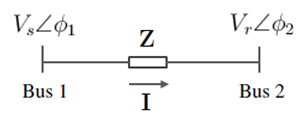
Figure 1. Simple AC power transmission model
Where  is the voltage and phase angle at the sending end
 is the voltage and phase angle at the receiving end
 is the complex impedance of the line.
 is the current phasor
The complex AC power transmitted to the receiving end bus can be calculated as follows:

At this stage, the impedance is purposely undefined and in the following sections, two different line impedance models will be introduced to illustrate the following fundamental features of AC power transmission:
- The power-angle relationship
- PV curves and steady-state voltage stability
Power-Angle Relationship
In its simplest form, we neglect the line resistance and capacitance and represent the line as purely inductive, i.e.  . The power transfer across the line is therefore:
![{\displaystyle {\boldsymbol {S}}={\boldsymbol {V_{r}}}\left[{\frac {{\boldsymbol {V_{s}}}-{\boldsymbol {V_{r}}}}{jX}}\right]^{*}}](https://wikimedia.org/api/rest_v1/media/math/render/svg/75bdfd710566de97a0745efd65ffdffbcb484525)


Where  is called the power angle, which is the phase difference between the voltages on bus 1 and bus 2.
We can see that active and reactive power transfer can be characterised as follows:


Plotting the active power transfer for various values of  , we get:
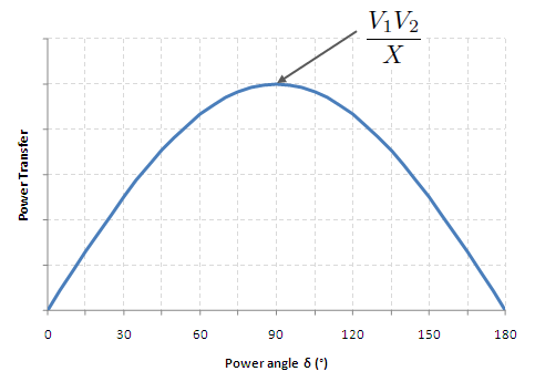
Figure 2. Active power transfer characteristic for a lossless line
The figure above is often used to articulate the Power-Angle Relationship. We can see that in this simple model, power will only flow when there is a phase difference between the voltages at the sending and receiving ends. Moreover, there is a theoretical limit to how much power can be transmitted through a line (shown here when the phase difference is 90o). This limit will be a recurring theme in these line models, i.e. lines have natural capacity limits on how much power they can transmit.
Steady-State Voltage Stability Limits
The lossless (L) line model can be made more realistic by adding a resistive component, i.e.  . The power transfer across the line is therefore:
![{\displaystyle {\boldsymbol {S}}={\boldsymbol {V_{r}}}\left[{\frac {{\boldsymbol {V_{s}}}-{\boldsymbol {V_{r}}}}{R+jX}}\right]^{*}}](https://wikimedia.org/api/rest_v1/media/math/render/svg/12263606d5d14f851ebd5f6888b0e1a36e06b008)


From the above equation, the active and reactive power transfer can be shown to be:


From the active power equation, we can solve for the voltage at bus 2 using the quadratic equation, i.e.:

Where 


By keeping the voltage at bus 1, power angle and line impedance constant, we can plot the effect of increasing the active power on the voltage at bus 2 on a PV curve:
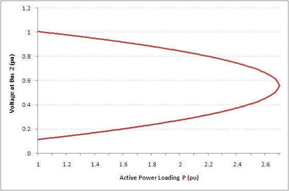
Figure 3. PV Curve at Bus 2 for a RL line
The PV curve shows that the voltage at bus 2 falls as the active power loading increases. The voltage falls until it hits a critical point (around 2.7pu loading) where the quadratic equation is no longer solvable. This is referred to as the "nose point" or "point of voltage collapse", and is the theoretical steady-state stability limit of the line.
Related Topics


