(diff) ← Older revision | Latest revision (diff) | Newer revision → (diff)
Motivation
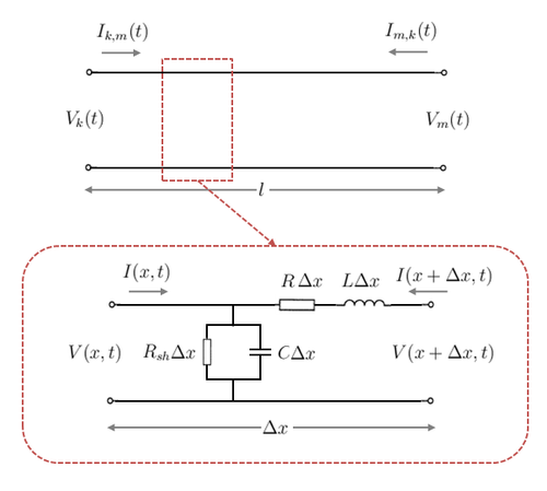
Figure 1. A generic single-phase distributed parameter line model
In this section, we try to answer the question - why bother with a model for frequency dependent lines?
Consider the generic single-phase distributed parameter line model of length  metres shown in Figure 1. Note that the model is represented as functions of both distance and time.
We can represent the series elements as an impedance and the shunt elements as an admittance as follows:


Where  is the series resistance (
 )
)
 is the series reactance ()
 is the shunt conductance (
 )
) is the shunt susceptance ()
If we only consider this model in the steady-state (i.e. the frequency domain), then time can be neglected and the model is exactly like the conventional single-phase distributed parameter line model.
Recall that the solution to the voltage and current of the steady-state model is as follows:
 ... Equ. (1)
 ... Equ. (2)
Where 

Things to note:
- 1) Voltage and current are complex phasors hence they are in bold.
- 2) The equations have slightly different signs to those derived in the distributed parameter line model. This is because the direction of current
 in Figure 3 is set in the opposite direction in this model.
We can add Equ. (1) to Equ. (2) to get:
 ... Equ. (3)
Similarly, we can subtract Equ. (2) from Equ. (1) to get:
 ... Equ. (4)
Re-arranging Equ. (3) and Equ. (4) to solve for the currents  and
and  :
:
 ... Equ. (5)
 ... Equ. (6)
From Fourier Transform theory, we know that multiplying by a complex exponential in the frequency domain is equivalent to a time shift in the time domain. Therefore, in the lossless case (i.e. R = G = 0.), the exponential part of  is:
is:

Where  is the travel time that we saw in the Bergeron model.
The characteristic impedance is also a scalar frequency-independent constant:

However if the line is not lossless, then we can see that the propagation constant and characteristic impedance are frequency dependent, i.e.
Since these quantities are complex and frequency dependent, the model does not simplify to a simple time shift in the time domain as we saw in the lossless case.
Moreover, the line parameters themselves are frequency dependent rather than constant across the full frequency range, i.e.  ,
,  ,
,  and
and  . Therefore, a constant parameter line model such as the Bergeron model is not suitable for cases where the frequency dependencies are significant (e.g. zero sequence impedances). This is the motivation for developing models that are able to capture the frequency dependencies of lines.
Single-Phase Lines
Multi-Conductor Lines
Related Topics

