Introduction
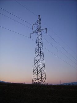
Figure 1. Three-phase, single-circuit tower line (image courtesy of
Wikipedia)
Single-phase equivalent line models (or positive-sequence line models) can be used quite accurately in three-phase systems when the system is balanced and the lines are perfectly transposed. However, when unbalanced systems or untransposed lines are being studied, these models break down and a full three-phase multi-conductor model is necessary.
Consider the three-phase, single circuit tower line in Figure 1, which shows three phase conductors and an earth wire. A segmental length of this multi-conductor system can be represented by the equivalent circuit in Figure 2 below:
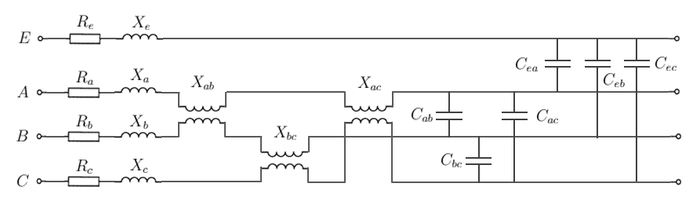
Figure 2. Circuit representation of a multi-conductor line segment
We can see that in a multi-conductor system, there is mutual coupling between the phase conductors (a, b and c), represented by the shunt inductances and capacitances. In the single-phase equivalent line model, these mutual couplings are ignored. Note that there could also be resistive coupling between phases, but is not shown in Figure 2 since resistive coupling is normally assumed to be negligible in overhead lines (i.e. shunt conductances = 0).
Recall that in the single-phase equivalent line model, we have single complex quantities for the series impedance  and shunt admittance
  of the line. But in the multi-conductor line, these single complex quantities are replaced by
  matrices, where n is the number of conductors in the system.
For example, the four conductor system in Figure 2 has the  impedance matrix:
![{\displaystyle [Z]=\left[{\begin{matrix}Z_{aa}&Z_{ab}&Z_{ac}&|&Z_{ae}\\Z_{ba}&Z_{bb}&Z_{bc}&|&Z_{be}\\Z_{ca}&Z_{cb}&Z_{cc}&|&Z_{ce}\\--&--&--&|&--\\Z_{ea}&Z_{eb}&Z_{ec}&|&Z_{ee}\end{matrix}}\right]\,}](https://wikimedia.org/api/rest_v1/media/math/render/svg/8b99df43a0ccf27e31891fa8be0e91d64209dfbc)
And the admittance matrix:
![{\displaystyle [Y]=\left[{\begin{matrix}Y_{aa}&Y_{ab}&Y_{ac}&|&Y_{ae}\\Y_{ba}&Y_{bb}&Y_{bc}&|&Y_{be}\\Y_{ca}&Y_{cb}&Y_{cc}&|&Y_{ce}\\--&--&--&|&--\\Y_{ea}&Y_{eb}&Y_{ec}&|&Y_{ee}\end{matrix}}\right]\,}](https://wikimedia.org/api/rest_v1/media/math/render/svg/cc5f732b4148fef09f52bc3039332455554e90eb)
Since we assume that under normal conditions, the earth wire is at zero potential (i.e. no voltage between the earth wire and neutral), we can use the Kron reduction to reduce the impedance and admittance matrices from to  matrices, i.e.
![{\displaystyle [Z']=\left[{\begin{matrix}Z_{aa}'&Z_{ab}'&Z_{ac}'\\Z_{ba}'&Z_{bb}'&Z_{bc}'\\Z_{ca}'&Z_{cb}'&Z_{cc}'\end{matrix}}\right]\,}](https://wikimedia.org/api/rest_v1/media/math/render/svg/802d90f7024edcb58c4d9f7d0b121cd67f4dbaa8)
![{\displaystyle [Y']=\left[{\begin{matrix}Y_{aa}'&Y_{ab}'&Y_{ac}'\\Y_{ba}'&Y_{bb}'&Y_{bc}'\\Y_{ca}'&Y_{cb}'&Y_{cc}'\end{matrix}}\right]\,}](https://wikimedia.org/api/rest_v1/media/math/render/svg/e32784657e8651f9c2a83eda8d50a943dca34af7)
We call these matrices the Kron reduced impedance and admittance matrices.
Nominal  Line
Line
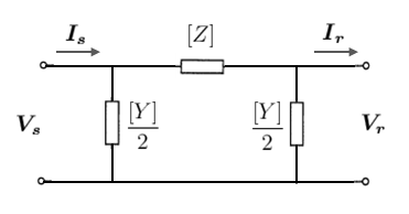
Figure 3. Multi-conductor nominal
line model
The multi-conductor nominal line model shown in Figure 3 is a direct substitution of the  complex parameters in the single-phase nominal Line with matrices.
If we consider the Kron reduced case, [Z] and [Y] are matrices as described in the previous section. The voltages and currents are  complex vectors of the form:
![{\displaystyle {\boldsymbol {V_{s}}}=\left[{\begin{matrix}{\boldsymbol {V_{s,a}}}\\{\boldsymbol {V_{s,b}}}\\{\boldsymbol {V_{s,c}}}\end{matrix}}\right]\,}](https://wikimedia.org/api/rest_v1/media/math/render/svg/159871f127c7f11473fbad809e40a7d9bd894a7e) ,
, ![{\displaystyle {\boldsymbol {I_{s}}}=\left[{\begin{matrix}{\boldsymbol {I_{s,a}}}\\{\boldsymbol {I_{s,b}}}\\{\boldsymbol {I_{s,c}}}\end{matrix}}\right]\,}](https://wikimedia.org/api/rest_v1/media/math/render/svg/b243daffa85185958254977cd9689fdd1505f2cb) ,
, ![{\displaystyle {\boldsymbol {V_{r}}}=\left[{\begin{matrix}{\boldsymbol {V_{r,a}}}\\{\boldsymbol {V_{r,b}}}\\{\boldsymbol {V_{r,c}}}\end{matrix}}\right]\,}](https://wikimedia.org/api/rest_v1/media/math/render/svg/32230420f9298a9623de6fdf8b3ca62b72d177ba) and
and ![{\displaystyle {\boldsymbol {I_{r}}}=\left[{\begin{matrix}{\boldsymbol {I_{r,a}}}\\{\boldsymbol {I_{r,b}}}\\{\boldsymbol {I_{r,c}}}\end{matrix}}\right]\,}](https://wikimedia.org/api/rest_v1/media/math/render/svg/9b7a16aa87a62fe2cfc39148b3094e4e3108de91)
The ABCD parameters of the multi-conductor nominal line are:
![{\displaystyle \left[{\begin{matrix}{\boldsymbol {V_{s}}}\\\\{\boldsymbol {I_{s}}}\end{matrix}}\right]=\left[{\begin{matrix}\left(I+{\frac {[Z][Y]}{2}}\right)&[Z]\\\\Y\left(I+{\frac {[Z][Y]}{4}}\right)&\left(I+{\frac {[Z][Y]}{2}}\right)\end{matrix}}\right]\left[{\begin{matrix}{\boldsymbol {V_{r}}}\\\\{\boldsymbol {I_{r}}}\end{matrix}}\right]\,}](https://wikimedia.org/api/rest_v1/media/math/render/svg/5d2a5a97ecdd8f652d14ba01e6ce32ef43bb3cd1)
Distributed Parameter Line
Refer to the distributed parameter model article for the detailed derivation of the model.
In the single-phase line model, we saw that it was possible to represent a distributed parameter line model using the same equivalent circuit as the nominal model, but with adjusted line parameters Z and Y. This was called the equivalent model and the adjusted parameters could be calculated as follows:


Where  is the propagation constant
However in the multi-conductor line, the propagation constant would be a matrix of the form:
![{\displaystyle [\gamma ]=\left([Z][Y]\right)^{\frac {1}{2}}}](https://wikimedia.org/api/rest_v1/media/math/render/svg/65734b2d97eb1ca0bb853a990bdfbd5a128f3757)
There is no straightforward method for calculating the hyperbolic sine and tangent functions of a matrix (the hyperbolic functions can be expanded as a Taylor series, but this is still not particularly easy to compute). This led to the development of the modal transformation, which is a method for decoupling the phases of the impedance and admittance matrices.
The ABCD parameters of the multi-conductor distributed parameter line are (in modal form):
![{\displaystyle \left[{\begin{matrix}{\boldsymbol {V_{s}'}}\\\\{\boldsymbol {I_{s}'}}\end{matrix}}\right]=\left[{\begin{matrix}\left[\cosh {(\gamma l)}\right]&\left[{\boldsymbol {Z_{c}}}\sinh {(\gamma l)}\right]\\\\\left[{\frac {1}{\boldsymbol {Z_{c}}}}\sinh {(\gamma l)}\right]&\left[\cosh {(\gamma l)}\right]\end{matrix}}\right]\left[{\begin{matrix}{\boldsymbol {V_{r}'}}\\\\{\boldsymbol {I_{r}'}}\end{matrix}}\right]\,}](https://wikimedia.org/api/rest_v1/media/math/render/svg/4ffdb4b3ae893964eb4665ffa176740d25bf84b9)
Where  ,
,  ,
,  and
and  are modal sending end and receiving end voltages and currents respectively:
![{\displaystyle {\boldsymbol {V_{s}'}}=\left[{\begin{matrix}{\boldsymbol {V_{s0}}}\\{\boldsymbol {V_{s1}}}\\{\boldsymbol {V_{s2}}}\end{matrix}}\right]\,}](https://wikimedia.org/api/rest_v1/media/math/render/svg/424eab880a48d758f5772c7133b5d5f3f831997f) ,
, ![{\displaystyle {\boldsymbol {I_{s}'}}=\left[{\begin{matrix}{\boldsymbol {I_{s0}}}\\{\boldsymbol {I_{s1}}}\\{\boldsymbol {I_{s2}}}\end{matrix}}\right]\,}](https://wikimedia.org/api/rest_v1/media/math/render/svg/2017071b74af7b86c85663714555e2a2220741de) ,
, ![{\displaystyle {\boldsymbol {V_{r}'}}=\left[{\begin{matrix}{\boldsymbol {V_{r0}}}\\{\boldsymbol {V_{r1}}}\\{\boldsymbol {V_{r2}}}\end{matrix}}\right]\,}](https://wikimedia.org/api/rest_v1/media/math/render/svg/dc249d85cf33254492ddf7c98b6a68598de778bc) and
and ![{\displaystyle {\boldsymbol {I_{r}'}}=\left[{\begin{matrix}{\boldsymbol {I_{r0}}}\\{\boldsymbol {I_{r1}}}\\{\boldsymbol {I_{r2}}}\end{matrix}}\right]\,}](https://wikimedia.org/api/rest_v1/media/math/render/svg/7e930c8d4edbee8e1955762d0a1f2c6fe4f5f87c)
The ABCD parameters are diagonal sub-matrices of the form:
![{\displaystyle \left[\cosh {(\gamma l)}\right]=\left[{\begin{matrix}\cosh {(\gamma _{0}x)}&&\\&\cosh {(\gamma _{1}x)}&\\&&\cosh {(\gamma _{2}x)}\end{matrix}}\right]}](https://wikimedia.org/api/rest_v1/media/math/render/svg/37d2d17e48d18884c8b4fc6f9c4f867103956e39) ,
, ![{\displaystyle \left[{\boldsymbol {Z_{c}}}\sinh {(\gamma l)}\right]=\left[{\begin{matrix}{\boldsymbol {Z_{0}}}\sinh {(\gamma _{0}x)}&&\\&{\boldsymbol {Z_{1}}}\sinh {(\gamma _{1}x)}&\\&&{\boldsymbol {Z_{2}}}\sinh {(\gamma _{2}x)}\end{matrix}}\right]}](https://wikimedia.org/api/rest_v1/media/math/render/svg/b4fb7378ebe285c60de68f249fd32ab328ab1d1c)
![{\displaystyle \left[{\frac {1}{\boldsymbol {Z_{c}}}}\sinh {(\gamma l)}\right]=\left[{\begin{matrix}{\frac {1}{\boldsymbol {Z_{0}}}}\sinh {(\gamma _{0}x)}&&\\&{\frac {1}{\boldsymbol {Z_{1}}}}\sinh {(\gamma _{1}x)}&\\&&{\frac {1}{\boldsymbol {Z_{2}}}}\sinh {(\gamma _{2}x)}\end{matrix}}\right]}](https://wikimedia.org/api/rest_v1/media/math/render/svg/00aaeb250715059b401f860a1728d3470af2dde1)
For details on the derivation of the modal equations, see the main distributed parameter model article.
References
Related Topics


