Bergeron Line Model

Introduction

The Bergeron line model is a discrete-time representation of the travelling wave model with constant line parameters that is conducive to computer implementation. The model takes its name from Louis Bergeron, who first the developed discrete-time models in the 1940s [1]. Prof. Hermann Dommel then applied the technique to the EMTP program in the late 1960s.

We first derive the Bergeron model for a lossless single-phase line and then explain why this model is unsuitable for a generic lossy line. We look at a workaround to represent lossy lines and lastly extend the model to multi-conductor lines.

Single Phase Lines

Lossless Lines

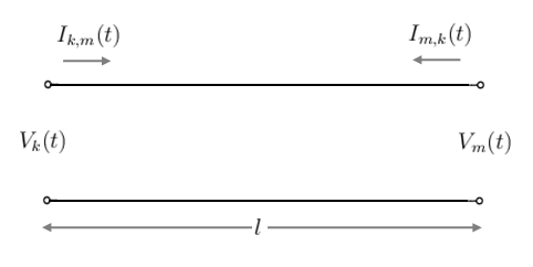
Consider a lossless single-phase transmission line of distance $l\,$ metres from starting node k and ending at node m, i.e.

Figure 1. Lossless single-phase line of length l

Recall from the travelling wave line model the following pair of voltage and current equations:

$I(x,t)=i^{+}(x-vt)+i^{-}(x+vt)\,$

$V(x,t)=Z_{c}\left[i^{+}(x-vt)-i^{-}(x+vt)\right]\,$

If we add $Z_{c}I(x,t)\,$ to the voltage equation, we get:

$V(x,t)+Z_{c}I(x,t)=2Z_{c}i^{+}(x-vt)\,$ ... Equ. (1)

Similarly, if we subtract $Z_{c}I(x,t)\,$ from the voltage equation, we get:

$V(x,t)-Z_{c}I(x,t)=-2Z_{c}i^{-}(x-vt)\,$ ... Equ. (2)

Looking at Equation (1), we can see that the left-hand side $V(x,t)+Z_{c}I(x,t)\,$ remains constant if $(x-vt)\,$ is also constant. Similarly for Equation (2), $V(x,t)-Z_{c}I(x,t)\,$ remains constant if $(x+vt)\,$ is also constant.

The key insight to the Bergeron model is this: $(x-vt)\,$ or $(x+vt)\,$ is constant to an observer that is travelling at the same constant speed $v\,$ and in the same direction as the travelling wave.

To prove this, consider the distance x travelled by an observer moving at the same speed and direction along the line as the travelling wave over some time t:

$x=x_{0}+vt\,$

Where $x_{0}\,$ is the starting location of the observer on the line. Re-arranging this equation, we can see that $x-vt=x_{0}\,$ is a constant.

Given the length of the line $l\,$ and speed $v\,$, we can calculate the travel time of the line $\tau \,$:

$\tau ={\frac {l}{v}}=l{\sqrt {LC}}\,$

Since it takes $\tau \,$ seconds for a waveform to travel the line from node k to node m, we can conclude that if an observer travelling with the forward travelling wave sees a value of $V+Z_{c}I\,$ as he leaves node k at time $(t-\tau )\,$, then the observer will see the same value when he arrives at node m at time $t\,$.

Mathematically, we get the following relationship between the nodes k and m:

$V_{k}(t-\tau )+Z_{c}I_{k,m}(t-\tau )=V_{m}(t)-Z_{c}I_{m,k}(t)\,$ ... Equ. (3)

(Note that the negative sign on the right hand side is simply to reflect the direction of current $I_{m,k}\,$ as shown in Figure 1).

Following the same logic for the backward travelling wave, we get:

$V_{m}(t-\tau )+Z_{c}I_{m,k}(t-\tau )=V_{k}(t)-Z_{c}I_{k,m}(t)\,$ ... Equ. (4)

We can re-arrange Equations (3) and (4) to solve for $I_{k,m}\,$ and $I_{m,k}\,$:

$I_{k,m}(t)={\frac {V_{k}(t)}{Z_{c}}}-{\frac {V_{m}(t-\tau )}{Z_{c}}}-I_{m,k}(t-\tau )\,$

$I_{m,k}(t)={\frac {V_{m}(t)}{Z_{c}}}-{\frac {V_{k}(t-\tau )}{Z_{c}}}-I_{k,m}(t-\tau )\,$

The above equations can be re-written as follows:

$I_{k,m}(t)={\frac {V_{k}(t)}{Z_{c}}}+I_{k}(t-\tau )\,$ ... Equ. (5)

$I_{m,k}(t)={\frac {V_{m}(t)}{Z_{c}}}+I_{m}(t-\tau )\,$ ... Equ. (6)

Where $I_{k}(t-\tau )=-{\frac {V_{m}(t-\tau )}{Z_{c}}}-I_{m,k}(t-\tau )\,$

and $I_{m}(t-\tau )=-{\frac {V_{k}(t-\tau )}{Z_{c}}}-I_{k,m}(t-\tau )\,$

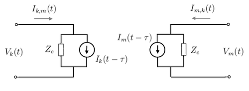
Notice that the expressions for $I_{k}(t-\tau )\,$ and $I_{m}(t-\tau )\,$ are composed of values from the past. This is precisely what makes the Bergeron model easy to implement in a computer program, since past values of voltage and current can be stored in memory as so-called "history vectors".

Lastly, the reason for re-writing the equations as above is so that we can represent Equations (5) and (6) as the Norton equivalent circuit in Figure 2 below.

Figure 2. Bergeron model equivalent circuit (single-phase line)

Generic Lines and how the Bergeron Model Breaks Down

Figure 3. A generic single-phase distributed parameter line model

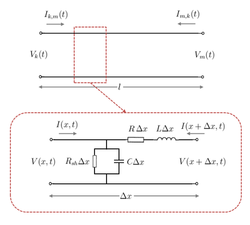
Consider the generic single-phase distributed parameter line model of length $l\,$ metres shown in Figure 3. Note that the model is represented as functions of both distance and time.

We can represent the series elements as an impedance and the shunt elements as an admittance as follows:

${\boldsymbol {z}}=R+j\omega L=R+jX\,$

${\boldsymbol {y}}={\frac {1}{R_{sh}}}+j\omega C=G+jB\,$

Where $R\,$ is the series resistance ($\Omega /m$)

$X\,$ is the series reactance ($\Omega /m$)

$G\,$ is the shunt conductance ($S/m$)

$B\,$ is the shunt susceptance ($S/m$)

If we only consider this model in the steady-state (i.e. the frequency domain), then time can be neglected and the model is exactly like the conventional single-phase distributed parameter line model.

Recall that the solution to the voltage and current of the steady-state model is as follows:

${\boldsymbol {V}}_{k}=\left({\frac {{\boldsymbol {V}}_{m}-{\boldsymbol {I}}_{m,k}{\boldsymbol {Z}}_{c}}{2}}\right)e^{{\boldsymbol {\gamma }}l}+\left({\frac {{\boldsymbol {V}}_{m}+{\boldsymbol {I}}_{m,k}{\boldsymbol {Z}}_{c}}{2}}\right)e^{-{\boldsymbol {\gamma }}l}\,$ ... Equ. (7)

${\boldsymbol {I}}_{k,m}{\boldsymbol {Z}}_{c}=\left({\frac {{\boldsymbol {V}}_{m}-{\boldsymbol {I}}_{m,k}{\boldsymbol {Z}}_{c}}{2}}\right)e^{\gamma l}-\left({\frac {{\boldsymbol {V}}_{m}+{\boldsymbol {I}}_{m,k}{\boldsymbol {Z}}_{c}}{2}}\right)e^{-\gamma l}\,$ ... Equ. (8)

Where ${\boldsymbol {\gamma }}={\sqrt {\boldsymbol {zy}}}={\sqrt {(R+j\omega L)(G+j\omega C)}}$

${\boldsymbol {Z}}_{c}={\sqrt {\boldsymbol {\frac {z}{y}}}}={\sqrt {\frac {(R+j\omega L)}{(G+j\omega C)}}}$

Things to note:

1) Voltage and current are complex phasors hence they are in bold.

2) The equations have slightly different signs to those derived in the distributed parameter line model. This is because the direction of current $I_{m,k}(t)\,$ in Figure 3 is set in the opposite direction in this model.

Like we did above in the lossless model, we can add Equ. (7) to Equ. (8) to get:

${\boldsymbol {V}}_{k}+{\boldsymbol {I}}_{k,m}{\boldsymbol {Z}}_{c}=\left({\boldsymbol {V}}_{m}-{\boldsymbol {I}}_{m,k}{\boldsymbol {Z}}_{c}\right)e^{{\boldsymbol {\gamma }}l}\,$ ... Equ. (9)

Similarly, we can subtract Equ. (8) from Equ. (7) to get:

${\boldsymbol {V}}_{k}-{\boldsymbol {I}}_{k,m}{\boldsymbol {Z}}_{c}=\left({\boldsymbol {V}}_{m}+{\boldsymbol {I}}_{m,k}{\boldsymbol {Z}}_{c}\right)e^{-{\boldsymbol {\gamma }}l}\,$ ... Equ. (10)

Re-arranging Equ. (9) and Equ. (10) to solve for the currents ${\boldsymbol {I}}_{m,k}\,$ and ${\boldsymbol {I}}_{k,m}\,$:

${\boldsymbol {I}}_{m,k}={\frac {{\boldsymbol {V}}_{m}}{{\boldsymbol {Z}}_{c}}}-{\frac {{\boldsymbol {V}}_{k}}{{\boldsymbol {Z}}_{c}}}e^{-{\boldsymbol {\gamma }}l}-{\boldsymbol {I}}_{k,m}e^{-{\boldsymbol {\gamma }}l}\,$ ... Equ. (11)

${\boldsymbol {I}}_{k,m}={\frac {{\boldsymbol {V}}_{k}}{{\boldsymbol {Z}}_{c}}}-{\frac {{\boldsymbol {V}}_{m}}{{\boldsymbol {Z}}_{c}}}e^{-{\boldsymbol {\gamma }}l}-{\boldsymbol {I}}_{m,k}e^{-{\boldsymbol {\gamma }}l}\,$ ... Equ. (12)

From Fourier Transform theory, we know that multiplying by a complex exponential in the frequency domain is equivalent to a time shift in the time domain. Therefore, the equations (11) and (12) above in the frequency domain can be made equivalent to equations (5) and (6) in the time domain if and only if the line is lossless, i.e. R = G = 0.

In the lossless case, the exponential part of $e^{-{\boldsymbol {\gamma }}l}\,$ is:

${\boldsymbol {\gamma }}l={\sqrt {\boldsymbol {zy}}}l={\sqrt {(j\omega L)(j\omega C)}}l=j\omega {\sqrt {LC}}l=j\omega \tau$

Where $\tau \,$ is the travel time that we calculated above.

The characteristic impedance is also a scalar frequency-independent constant:

${\boldsymbol {Z}}_{c}={\sqrt {\boldsymbol {\frac {z}{y}}}}={\sqrt {\frac {(j\omega L)}{(j\omega C)}}}={\sqrt {\frac {L}{C}}}$

However if the line is not lossless, then we can see that the propagation constant and characteristic impedance are frequency dependent, i.e.

${\boldsymbol {\gamma }}={\sqrt {\boldsymbol {zy}}}={\sqrt {(R+j\omega L)(G+j\omega C)}}$

${\boldsymbol {Z}}_{c}={\sqrt {\boldsymbol {\frac {z}{y}}}}={\sqrt {\frac {(R+j\omega L)}{(G+j\omega C)}}}$

Since these parameters are complex and frequency dependent, the model does not simplify to a simple time shift in the time domain as we saw in the lossless case, i.e. the signals are attenuated and distorted in the lossy case. Therefore the Bergeron model cannot be used for the generic (lossy) distributed parameter line and a frequency dependent line model is required.

Workaround for Lossy Lines

We saw above that the Bergeron model doesn't work for lossy distributed parameter lines. However, we can work around this limitation by assuming that the shunt conductances are negligible and the series resistances are lumped at the ends of the line and in the middle. The line is therefore modelled as two lossless Bergeron equivalent circuits with lumped resistances at the middle and ends (see Figure 4 below).

Figure 4. Bergeron model for a lossy line

This workaround model is reasonably accurate when ${\frac {R}{4}}<<Z_{c}\,$. However, if this doesn't hold (for example, at very high frequencies when skin effects lead to high resistances) and/or shunt conductances are significant, then the line needs to be broken down into smaller sections.

Multi-Conductor Lines

Lossless Lines

As described in the article on the travelling wave model, the single-phase lossless line can be extended to a multi-conductor line by using a modal transformation to decouple the phases. The resulting modal (012) quantities form three decoupled Bergeron equivalent circuits that can be then solved independently. Finally, the parameters are transformed back to the phase domain. Figure 5 shows how the multi-conductor Bergeron model is structured.

Figure 5. Multi-conductor lossless Bergeron model

Lossy Lines

Like in the single-phase case, the multi-conductor Bergeron model is not suitable for generic lossy lines and a workaround must be used where series resistances are lumped at the middle and ends of the line. Note that the shunt conductance G is still assumed to be negligible.

References

• [1] Bergeron, Louis Jean Baptiste "Du Coup de Bélier en Hydraulique - Au Coup de Foudre en Electricité (Waterhammer in hydraulics and wave surges in electricity)", 1950, Paris: Dunod (in French) (English translation by ASME Committee, New York: John Wiley & Sons, 1961.)

Related Topics

• Overhead Line Models
• Travelling Wave Line Model
• Distributed Parameter Line Model
• Frequency Dependent Line Model