ABCD Parameters (Generalised Line Constants)
Consider the overhead line represented as a two-port network of the form:
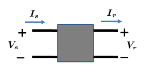
Figure 1. Two-port network representation
Where  is the voltage at the sending end
 is the voltage at the receiving end
 is the current at the sending end
 is the current at the receiving end
Suppose the system can be represented such that the sending end quantities can be written as a linear function of the receiving end quantities, i.e.


Where that the parameters  ,
,  ,
,  and
and  are constants (which can be either real or complex). These constants are called the ABCD parameters of the line. Sometimes, they are referred to as Generalised Line Constants.
In matrix form, the ABCD parameters are represented as follows:
![{\displaystyle \left[{\begin{matrix}{\boldsymbol {V_{s}}}\\{\boldsymbol {I_{s}}}\end{matrix}}\right]=\left[{\begin{matrix}A&C\\B&D\end{matrix}}\right]\left[{\begin{matrix}{\boldsymbol {V_{r}}}\\{\boldsymbol {I_{r}}}\end{matrix}}\right]\,}](https://wikimedia.org/api/rest_v1/media/math/render/svg/2d1a37cae435cc17d1e2f76e4da70426eff0bba6)
Lossless (L) Line
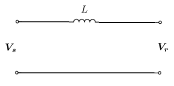
Figure 2. Lossless line model
In its simplest form, we neglect the line resistance and capacitance and represent the line as purely inductive, i.e. the line impedance  .
.
Analysing this circuit using Kirchhoff's laws, we get:


Therefore the ABCD parameters of the lossless (L) line in matrix form are:
![{\displaystyle \left[{\begin{matrix}{\boldsymbol {V_{s}}}\\{\boldsymbol {I_{s}}}\end{matrix}}\right]=\left[{\begin{matrix}1&X_{L}\\0&1\end{matrix}}\right]\left[{\begin{matrix}{\boldsymbol {V_{r}}}\\{\boldsymbol {I_{r}}}\end{matrix}}\right]\,}](https://wikimedia.org/api/rest_v1/media/math/render/svg/6fc4a72f74284ce7473bf7d1f46483d889e7e38a)
RL Line
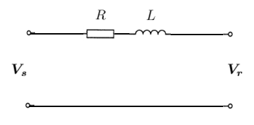
Figure 3. RL line model
The lossless (L) line model can be made more realistic by adding a resistive component, i.e.  .
.
Using the same logic as the lossless (L) line above, the sending end quantities can be calculated as:

Therefore the ABCD parameters of the RL line in matrix form are:
![{\displaystyle \left[{\begin{matrix}{\boldsymbol {V_{s}}}\\{\boldsymbol {I_{s}}}\end{matrix}}\right]=\left[{\begin{matrix}1&{\boldsymbol {Z}}\\0&1\end{matrix}}\right]\left[{\begin{matrix}{\boldsymbol {V_{r}}}\\{\boldsymbol {I_{r}}}\end{matrix}}\right]\,}](https://wikimedia.org/api/rest_v1/media/math/render/svg/482d16d3dcba656634292866ed7d4f2c1b851fa6)
Lossless (LC) Line
We've so far neglected capacitances in our line, but at higher voltages and longer line lengths, the effect of shunt capacitances becomes more significant. So we now consider a lossless LC line of the form:
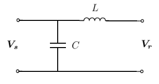
Figure 4. Lossless (LC) transmission line model
The inductance and capacitance can be represented as a reactance and susceptance as follows:


Analysing this circuit using Kirchhoff's laws, we get:


Therefore the ABCD parameters of the LC line in matrix form are:
![{\displaystyle \left[{\begin{matrix}{\boldsymbol {V_{s}}}\\{\boldsymbol {I_{s}}}\end{matrix}}\right]=\left[{\begin{matrix}1&X_{L}\\Y_{C}&1+X_{L}Y_{C}\end{matrix}}\right]\left[{\begin{matrix}{\boldsymbol {V_{r}}}\\{\boldsymbol {I_{r}}}\end{matrix}}\right]\,}](https://wikimedia.org/api/rest_v1/media/math/render/svg/667e2482fe355fa13f66aaa699e09c8a087f319e)
Nominal  Line
Line
The so-called "Nominal " model is an extension of the lossless LC line where a series resistance is added and the shunt capacitances are balanced (i.e. half at each end of the line).
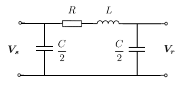
Figure 5. Nominal
transmission line model
The series elements can be represented as an impedance and the shunt capacitances as susceptances as follows:

Before we analyse the circuit, it is worth noting from Kirchhoff's current law that the current across the series impedance  is:
is:

Analysing this circuit using Kirchhoff's laws, we get:

Substituting in  :
:


![{\displaystyle ={\frac {\boldsymbol {Y}}{2}}\left[\left(1+{\frac {{\boldsymbol {Z}}{\boldsymbol {Y}}}{2}}\right){\boldsymbol {V_{r}}}+{\boldsymbol {Z}}{\boldsymbol {I_{r}}}\right]+{\frac {\boldsymbol {Y}}{2}}{\boldsymbol {V_{r}}}+{\boldsymbol {I_{r}}}\,}](https://wikimedia.org/api/rest_v1/media/math/render/svg/5a623fff7bf3edfacc4414deebc675999e328bf3)

Therefore the ABCD parameters of the nominal line in matrix form are:
![{\displaystyle \left[{\begin{matrix}{\boldsymbol {V_{s}}}\\\\{\boldsymbol {I_{s}}}\end{matrix}}\right]=\left[{\begin{matrix}\left(1+{\frac {{\boldsymbol {Z}}{\boldsymbol {Y}}}{2}}\right)&{\boldsymbol {Z}}\\\\{\boldsymbol {Y}}\left(1+{\frac {{\boldsymbol {Z}}{\boldsymbol {Y}}}{4}}\right)&\left(1+{\frac {{\boldsymbol {Z}}{\boldsymbol {Y}}}{2}}\right)\end{matrix}}\right]\left[{\begin{matrix}{\boldsymbol {V_{r}}}\\\\{\boldsymbol {I_{r}}}\end{matrix}}\right]\,}](https://wikimedia.org/api/rest_v1/media/math/render/svg/30037233f72131ca9e31dd179b0d6ae1fb75992e)
Distributed Parameter Line
Refer to the distributed parameter model article for the detailed derivation of the model.
The models above have been "lumped", such that the line has been represented by lumped R, L and C elements. However in reality, the R, L and C elements are distributed along the length of the line. So now let's consider a distributed parameter model where the voltage and current at any point  along the line (relative to the receiving end bus) are given by the following equations:


Where  is the propagation constant (
 )
)
 is the characteristic impedance (
 )
)
Note that the equations above are derived here.
By inspection, the ABCD parameters of the above equations can be represented in matrix form (for a line of length  metres) as follows:
![{\displaystyle \left[{\begin{matrix}{\boldsymbol {V_{s}}}\\\\{\boldsymbol {I_{s}}}\end{matrix}}\right]=\left[{\begin{matrix}\cosh({\boldsymbol {\gamma }}l)&{\boldsymbol {Z}}_{c}\sinh({\boldsymbol {\gamma }}l)\\\\{\frac {1}{{\boldsymbol {Z}}_{c}}}sinh({\boldsymbol {\gamma }}l)&\cosh({\boldsymbol {\gamma }}l)\end{matrix}}\right]\left[{\begin{matrix}{\boldsymbol {V_{r}}}\\\\{\boldsymbol {I_{r}}}\end{matrix}}\right]\,}](https://wikimedia.org/api/rest_v1/media/math/render/svg/84c751fe40fbb9e608b1835a0512c90917157eaa)
Equivalent Line
The "equivalent " line model is essentially a line model with the same circuit structure as the nominal line (i.e. Figure 5), but the ABCD parameters of the distributed parameter line. In order to get the same ABCD parameters as the distributed parameter line, the nominal line impedance and admittance  need to be adjusted such that:
![{\displaystyle \left[{\begin{matrix}A&C\\B&D\end{matrix}}\right]=\left[{\begin{matrix}\left(1+{\frac {{\boldsymbol {Z'}}{\boldsymbol {Y'}}}{2}}\right)&{\boldsymbol {Z'}}\\\\{\boldsymbol {Y'}}\left(1+{\frac {{\boldsymbol {Z'}}{\boldsymbol {Y'}}}{4}}\right)&\left(1+{\frac {{\boldsymbol {Z'}}{\boldsymbol {Y'}}}{2}}\right)\end{matrix}}\right]=\left[{\begin{matrix}\cosh({\boldsymbol {\gamma }}l)&{\boldsymbol {Z}}_{c}\sinh({\boldsymbol {\gamma }}l)\\\\{\frac {1}{{\boldsymbol {Z}}_{c}}}sinh({\boldsymbol {\gamma }}l)&\cosh({\boldsymbol {\gamma }}l)\end{matrix}}\right]\,}](https://wikimedia.org/api/rest_v1/media/math/render/svg/3ee0f15e9f1a3f8dc9742dfbb364838fb7e3c630)
Where  and
and  are the adjusted line impedance and admittance respectively (see conversion from nominal values below)
- is the length of the line (m)
- is the propagation constant ()
- is the characteristic impedance ()
The adjusted line parameters can be calculated from the nominal line parameters as follows:
![{\displaystyle {\boldsymbol {Z'}}=\left[{\frac {\sinh({\boldsymbol {\gamma }}l)}{{\boldsymbol {\gamma }}l}}\right]{\boldsymbol {Z}}}](https://wikimedia.org/api/rest_v1/media/math/render/svg/cf763b46d7f4ebe98c0f5571ffc21a6375481d2f)
![{\displaystyle {\frac {\boldsymbol {Y'}}{2}}=\left[{\frac {\tanh \left({\frac {{\boldsymbol {\gamma }}l}{2}}\right)}{\frac {{\boldsymbol {\gamma }}l}{2}}}\right]{\frac {\boldsymbol {Y}}{2}}}](https://wikimedia.org/api/rest_v1/media/math/render/svg/bce83319486bb351d490e5b2306d866bdd67720b)
Alternatively, the adjusted line parameters can also be represented as follows:


Click here for the full derivation of the calculation of the adjusted line parameters, including the alternative representation.
Related Topics


